Auxilliary Networks - Neural Injective Geometry

We now introduce, Auxilliary Networks, additions to the basic Injective Network architecture that enhances their representation power.

# Basic imports
import torch
from torch import nn
import geosimilarity as gs
from NIGnets import NIGnet

from assets.utils import automate_training, plot_curves

Pre-Auxilliary Networks¶

Closed Condition: A Closer Look¶

Let’s first try fitting an Injective Network to a square using the PReLU function. Indeed as discussed before the PReLU activation does not guarantee non-self-intersection but we use it to gain insights.

from assets.shapes import square

# Generate target curve points
num_pts = 1000
t = torch.linspace(0, 1, num_pts).reshape(-1, 1)
Xt_square = square(num_pts)

square_net = NIGnet(layer_count = 3, act_fn = nn.PReLU)
automate_training(
    model = square_net, loss_fn = gs.MSELoss(), X_train = t, Y_train = Xt_square,
    learning_rate = 0.1, epochs = 1000, print_cost_every = 200
)

Xp_square = square_net(t)
plot_curves(Xp_square, Xt_square)

Epoch: [   1/1000]. Loss:    1.052965
Epoch: [ 200/1000]. Loss:    0.006894
Epoch: [ 400/1000]. Loss:    0.006118
Epoch: [ 600/1000]. Loss:    0.005084
Epoch: [ 800/1000]. Loss:    0.003844
Epoch: [1000/1000]. Loss:    0.003531

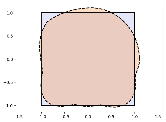
We observe that the fit is really bad.

This is because the network first transforms the interval $t\in [0, 1]$ to a circle and then deeper layers try to transform that to a square. This is not an easy task as the network has to transform the circle arcs to the four straight edges.

Let’s have a look at the first transformation as discussed in the section Condition 2 - Closed Curves:

C(t) = \begin{bmatrix} cos(2\pi t)\\ sin(2\pi t) \end{bmatrix}

(1)

The point $[\cos(2\pi t), \sin(2\pi t)]$ is a point on the unit circle centered at the origin. What is happening here is that the open interval $t \in [0, 1]$ is transformed to a circle that makes sure that the first and the last point are the same and when fed into the network lead to the same output point and hence create closed curves. This is explained visually in Figure 4.

Transforming the line segment [0, 1] to the unit circle centered at the origin. — Figure 4:Transforming the line segment $[0, 1]$ to the unit circle centered at the origin.

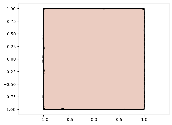
We could have also achieved the closed condition by transforming to a square instead of a circle. For the above problem of fitting to a square this should help immensely as the Injective Network has to learn the identity mapping only! This is easy to do when using the PReLU activation.

Code for transforming

[0, 1]

to unit square

shapes.py

def square_from_t(t: torch.Tensor) -> torch.Tensor:
    # Generate theta values corresponding to t
    theta = 2 * torch.pi * t.reshape(-1)
    
    x, y = torch.cos(theta), torch.sin(theta)
    s = torch.maximum(torch.abs(x), torch.abs(y))
    x_sq, y_sq = x/s, y/s

    X = torch.stack([x_sq, y_sq], dim = 1)
    return X

from assets.shapes import square_from_t

class InjectiveNet_SquareClosed(nn.Module):
    def __init__(self, layer_count, act_fn):
        super().__init__()

        # Transform from t on the [0, 1] interval to unit square for closed shapes
        self.closed_transform = square_from_t

        layers = []
        for i in range(layer_count):
            layers.append(nn.Linear(2, 2))
            layers.append(act_fn())
        
        self.linear_act_stack = nn.Sequential(*layers)
    
    def forward(self, t):
        x = self.closed_transform(t)
        x = self.linear_act_stack(x)
        return x

# Generate target curve points
num_pts = 1000
t = torch.linspace(0, 1, num_pts).reshape(-1, 1)
X_t_square = square(num_pts)

square_net = InjectiveNet_SquareClosed(layer_count = 1, act_fn = nn.PReLU)
automate_training(
    model = square_net, loss_fn = gs.MSELoss(), X_train = t, Y_train = X_t_square,
    learning_rate = 0.1, epochs = 1000, print_cost_every = 200
)

X_p_square = square_net(t)
plot_curves(X_p_square, X_t_square)

# Print model parameters after learning
for name, param in square_net.named_parameters():
    print(f"Layer: {name} | Values : {param[:2]} \n")

Epoch: [   1/1000]. Loss:    0.579582
Epoch: [ 200/1000]. Loss:    0.000000
Epoch: [ 400/1000]. Loss:    0.000000
Epoch: [ 600/1000]. Loss:    0.000000
Epoch: [ 800/1000]. Loss:    0.000000
Epoch: [1000/1000]. Loss:    0.000000

Layer: linear_act_stack.0.weight | Values : tensor([[1.0000e+00, 1.6361e-08],
        [2.4072e-09, 1.0000e+00]], grad_fn=<SliceBackward0>) 

Layer: linear_act_stack.0.bias | Values : tensor([-1.3566e-07, -6.1809e-08], grad_fn=<SliceBackward0>) 

Layer: linear_act_stack.1.weight | Values : tensor([1.0000], grad_fn=<SliceBackward0>)

Observe above that the network indeed learns the identity mapping as the linear transformation matrix ends up as the identity matrix and the PReLU activation function ends up as $x$ that is the identity map with the slope as 1 and bias being 0.

Pre-Auxilliary Network¶

Indeed we could have transformed to any simple closed curve first and then attached the neural network layers after that. But since representing general simple closed curves is what we are trying to achieve, we can do a simpler thing. We transform the interval $[0, 1]$ to a closed loop represented through polar coordinates in the form:

r = f(\theta), \quad \theta \in [0, 2\pi)

(2)

where $\theta = 2\pi t$ with $t$ in $[0, 1]$ .

We can then use the vector $[r \cos(\theta), r \sin(\theta)]^{T}$ as the first layer and attach the usual Injective Network layers on top. This transformation from $t$ to the vector $[r \cos(\theta), r \sin(\theta)]^{T}$ is injective and satisfies the condition $F(0) = F(1)$ and thus will create closed curves.

The function $f$ can be represented using a full neural network with no additional constraints except that the output has to be positive. We call this network the Pre-Auxilliary Network.

The basic idea is that the Pre-Auxilliary Network will provide a favorable initial shape to the Injective Network and make its learning task simpler.

Using Pre-Auxilliary Networks with NIGnets is really simple! Just create an appropriate network and pass that to the NIGnets constructor. We demonstrate this below.

The power of PreAux nets lies in the fact that a full scale MLP can be used to represent them. But a few conditions must be met to create a valid PreAux Net:

class PreAuxNet(nn.Module):
    def __init__(self, layer_count, hidden_dim):
        super().__init__()

        # Pre-Auxilliary net needs closed transform to get same r at theta = 0, 2pi
        self.closed_transform = lambda t: torch.hstack([
            torch.cos(2 * torch.pi * t),
            torch.sin(2 * torch.pi * t)
        ])

        layers = [nn.Linear(2, hidden_dim), nn.ReLU()]
        for i in range(layer_count):
            layers.append(nn.Linear(hidden_dim, hidden_dim))
            layers.append(nn.ReLU())
        layers.append(nn.Linear(hidden_dim, 1))
        layers.append(nn.ReLU())

        self.forward_stack = nn.Sequential(*layers)
    
    def forward(self, t):
        unit_circle = self.closed_transform(t) # Rows are cos(theta), sin(theta)
        r = self.forward_stack(unit_circle)
        x = r * unit_circle # Each row is now r*cos(theta), r*sin(theta)
        return x

from assets.shapes import square

# Generate target curve points
num_pts = 1000
t = torch.linspace(0, 1, num_pts).reshape(-1, 1)
Xt_square = square(num_pts)

preaux_net = PreAuxNet(layer_count = 3, hidden_dim = 10)
square_net = NIGnet(layer_count = 1, act_fn = nn.PReLU, preaux_net = preaux_net)
automate_training(
    model = square_net, loss_fn = gs.MSELoss(), X_train = t, Y_train = Xt_square,
    learning_rate = 0.1, epochs = 1000, print_cost_every = 200
)

Xp_square = square_net(t)
plot_curves(Xp_square, Xt_square)

Epoch: [   1/1000]. Loss:    0.976244
Epoch: [ 200/1000]. Loss:    0.000039
Epoch: [ 400/1000]. Loss:    0.000025
Epoch: [ 600/1000]. Loss:    0.000031
Epoch: [ 800/1000]. Loss:    0.000035
Epoch: [1000/1000]. Loss:    0.000036

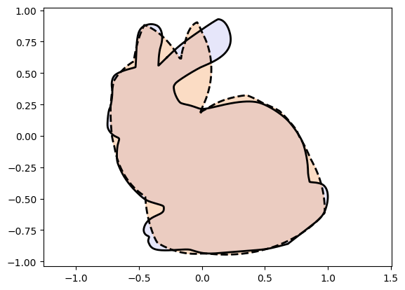
Great! Using a Pre-Auxilliary Network helps us build an Injective Network on top of a favorable closed transform. This therefore helps us cover both the circle and the square fitting cases without specifying a particular initial transform such as the circle or square. Pre-Auxilliary Networks are therefore a way of adding to the capacity of Injective Networks using full scale neural networks.

from assets.shapes import stanford_bunny

# Generate target curve points
num_pts = 1000
t = torch.linspace(0, 1, num_pts).reshape(-1, 1)
Xt_bunny = stanford_bunny(num_pts)

preaux_net = PreAuxNet(layer_count = 2, hidden_dim = 50)
bunny_net = NIGnet(layer_count = 1, act_fn = nn.PReLU, preaux_net = preaux_net)
automate_training(
    model = bunny_net, loss_fn = gs.MSELoss(), X_train = t, Y_train = Xt_bunny,
    learning_rate = 0.1, epochs = 1000, print_cost_every = 200
)

Xp_bunny = bunny_net(t)
plot_curves(Xp_bunny, Xt_bunny)

Epoch: [   1/1000]. Loss:    0.550154
Epoch: [ 200/1000]. Loss:    0.005555
Epoch: [ 400/1000]. Loss:    0.004586
Epoch: [ 600/1000]. Loss:    0.004364
Epoch: [ 800/1000]. Loss:    0.004427
Epoch: [1000/1000]. Loss:    0.004183

We now look at another technique that allows us to use full scale neural networks to augment the power of Injective Networks.

Post-Auxilliary Networks¶

More Representation Power: Augmenting in Polar Coordinates¶

The Injective Network architecture can represent simple closed curves. But as we saw the requirement of network injectivity for imparting non-self-intersection to the parameterization restricted the hidden layer size to 2. Therefore the only thing we can control for increasing representation power is the network depth.

There is a way of working with polar coordinates where we can post-augment the parameterization with a general neural network giving a boost to representation power. We discuss this technique now. But first we need to discuss the polar version of the Injective Network.

Polar Neural Injective Geometry¶

Consider first a polar setup of the parameterization similar to the cartesian case:

\begin{align*} r &= f(t)\\ \theta &= g(t), \quad t \in [0, 1) \end{align*}

(3)

Again as before we look at a vector-valued equivalent:

F: t \rightarrow \begin{bmatrix} r\\ \theta \end{bmatrix}

(4)

We use the same network architecture as before with the only difference that now the output is $[r, \theta]^{T}$ :

Figure showing a neural network architecture for polar representation of simple closed curves. — Figure 2:The network architecture for polar representation of simple closed curves looks deceptively similar to the one for cartesian coordinates with only the interpretation of the outputs being $[r, \theta]^{T}$ instead of $[x, y]^{T}$ . But for the polar representation we need more constraints to hold to guarantee simple closed curves.

The network architecture for the polar representation looks deceptively similar to the one for cartesian coordinates with only the interpretation of the outputs being $[r, \theta]^{T}$ instead of $[x, y]^{T}$ . But for the polar representation we need additional constraints to hold to guarantee simple closed curves.

Positive $r$

The polar representation requires that $r$ is positive. The above architecture by default puts no restriction on what values $r$ can take. To generate only positive $r$ values the activation function used at the last layer should be such that its outputs are always positive. Note that this activation function should still be injective. Valid activation functions include $sigmoid$ , $softplus$ , modified $tanh$ or $ELU$ etc. An example modification of $tanh$ would be to add 1 to it and use $tanh(x) + 1$ as the final activation function, this works as $tanh$ is injective with range $(-1, 1)$ .

Restricting $\theta \in [0, 2 \pi)$

Once we make sure that we choose the right activation function that only outputs positive values we need to make sure of the range of θ for a couple of reasons:

The first is related to self-intersection. The mapping from $t \to [r, \theta]$ is injective. But the curve it may trace out in the current form may self-intersect. Consider as an e.g. the points $[1, \pi]$ and $[1, 3\pi]$ . These are different outputs and does not violate injectivity of the network but they correspond to the same point in the plane!
The second one is a representation problem. Let’s say we use the last layer activation function to be $tanh + 1$ . This function has the range $(0, 2)$ and therefore this will also be the possible θ that we can generate. Thus, our curves will all be limited to $\theta \in (0, 2)$ . Of course, this is an artifact of using $tanh + 1$ and a different activation function like the $ELU + 1$ would not have this issue, but it will suffer from the first issue above.

Therefore the possible activation functions we can use at the last layer must be restricted to those that can further be scaled to have a range $[0, 2\pi)$ . One valid choice would be the function $2\pi(tanh + 1)$ .

Note: There is then also the concern on the range of r.

Post-Auxilliary Networks¶

Now consider a polar representation of the form:

r = h(\theta), \quad \theta \in [0, 2\pi)

(5)

As we discussed before this is a guaranteed non-self-intersecting representation but suffers from the general curve representation problem discussed in the section Naive Usage of Polar Coordinates: The Representation Power Problem.

But this can be a very powerful representation as we can use a full scale neural network to parameterize $f(\theta)$ . We now see a way of combining the injective polar representation with this parameterization.

Note: The final activation function of the neural network should be chosen such that the outputs are always positive to agree with $r$ being positive.

Probably the simplest thing to do would be to simply add the outputs of the two networks. One would do this by adding the $r$ value output from the auxilliary network to the different $r$ values that are output from the injective network at any given θ. But performing this directly has a problem. The auxilliary network is defined at all θ by definition but the injective network may not output some values of θ and therefore we cannot add the two. This is shown in Figure 3.

But there is a simple way of bypassing this problem. The basic idea is to use $r$ values only at $t$ values that lead to valid θ. The valid θ are generated as $g(t)$ . Therefore the corresponding $r = h(\theta) = h(g(t))$ are the $r$ values generated at valid θ that occur as $t$ is traversed from $[0, 1)$ .

Consider a vector-valued mapping associated with the auxilliary network:

A: t \rightarrow \begin{bmatrix} h(g(t))\\ 0 \end{bmatrix}

(6)

Note this requires that we first feed in $t$ into the injective network, get the corresponding θ and then feed that into the auxilliary network to generate the $r$ for the $A$ mapping.

We now have the following two vector-valued mappings:

F: t \rightarrow \begin{bmatrix} f(t)\\ g(t) \end{bmatrix} \quad A: t \rightarrow \begin{bmatrix} h(g(t))\\ 0 \end{bmatrix}

(7)

Consider the addition of these:

F + A: t \rightarrow \begin{bmatrix} f(t) + h(g(t))\\ g(t) \end{bmatrix}

(8)

We now need to prove that this mapping generates simple closed curves. This is quite intuitive and the proof is as follows:

Closed: The curves will be closed if $(F + A)(0) = (F + A)(1)$ . But we have $F(0) = F(1)$ as $F$ is the injective network. That is,
$(f(0), g(0)) = (f(1), g(1))$
(9)
We have $A(0) = (h(g(0)), 0)$ and $A(1) = (h(g(1)), 0)$ . Now since $g(0) = g(1)$ we also have $A(0) = A(1)$ and hence the curves will be closed.
Simple: The curves will be simple if the mapping $F + A$ is injective. Which is true if:
$t_1 \neq t_2 \implies (F + A)(t_1) \neq (F + A)(t_2)$
(10)
We start with the assumption that $F + A$ is not injective. That is for some $t_1$ and $t_2$ the outputs are the same. Then we have:
$\begin{align*} g(t_1) &= g(t_2) \end{align*}$
(11)
and
$\begin{align*} &f(t_1) + h(g(t_1)) = f(t_2) + h(g(t_2)) \\ \implies &f(t_1) + h(g(t_1)) = f(t_2) + h(g(t_1)) \\ \implies &f(t_1) = f(t_2) \end{align*}$
(12)
But this means that $F(t_1) = F(t_2)$ which is a contradiction as $F$ is the injective network. Therefore our original assumption that $F + A$ is not injective is false, and we conclude that the mapping $F + A$ is indeed injective.

Figure 4 shows the architecture for the augmented network

Combination of the injective network and the auxilliary network in the correct way. — Figure 4:First $t$ is fed into the injective network to obtain its $r_i$ and $\theta_i$ output. This $\theta_i$ is then fed into the auxilliary network to generate $r_a$ which is then added to $r_i$ to generate the final value.