Injective Networks - Neural Injective Geometry

Please click the power ⏻ button to start a kernel to be able to execute code on this webpage. To start a separate binder notebook click the rocket icon on the top.

To run code cells click the ▶ button available on the right side of code cells upon hover (when a kernel is running).

Make sure to run the cells below to install dependencies.

# To experience basic features
%pip install numpy
%pip install matplotlib
%pip install ipywidgets

# If you want to do in-browser network training
%pip install svg.path
%pip install torch

Neural Injective Curves¶

We now discuss the abstract idea behind our shape parameterization to represent general simple closed curves in the plane. As we shall see, this approach is conceptual and to actually create curves a construction method is needed. Our method is based on neural networks with special architectures that work as construction methods. We will see that the basic neural network architecture is a very natural approach for constructing non-self-intersecting curves.

Cartesian Neural Injective Curves¶

Consider the following parameterization to represent curves:

\begin{align*} x &= f(t)\\ y &= g(t), \quad t \in [0, 1] \end{align*}

(1)

This representation can potentially represent any curve in the plane not necessarily simple and closed. Thus it is too broad, we want the functions $f$ and $g$ to be such that we only represent simple and closed curves. Refer Figure 1 for a visual understanding of simple closed curves.

Four types of curves: simple/not simple + closed/not closed — Figure 1:We will be concerned with simple closed curves, i.e. curves that loop back and do not self-intersect.

Simple: A curve is simple if it does not self-intersect. That is, two different $t$ values should not map to the same point in the plane. Mathematically,
$t_1 \neq t_2 \implies (x(t_1), y(t_1)) \neq (x(t_2), y(t_2))$
(2)
Closed: A curve is closed if the starting and the ending points are the same. Mathematically,
$(x(0), y(0)) = (x(1), y(1))$
(3)

If these additional constraints are satisfied by the functions $f$ and $g$ then the curves generated will be guaranteed to be simple closed curves. We now discuss a way of constructing functions $f$ and $g$ such that they always satisfy these constraints.

To create a construction mechanism we need to first look at the problem differently through a single vector-valued mapping instead of two scalar-valued functions $f$ and $g$ . Consider also, instead of two scalar values $x$ and $y$ , a single vector which has the two values stacked $[x, y]^{T}$ . This vector is parameterized as before through a parameter $t$ . Concretely, consider a vector-valued mapping $F$ that maps $t$ to the vector of $x$ and $y$ .

F: t \rightarrow \begin{bmatrix} x\\ y \end{bmatrix}

(4)

Condition 1 - Simple Curves¶

For the curves represented through the mapping $F$ to be simple, we need $F$ to be an injective map as then every $t$ value will map to a different point in the plane and does not self-intersect. We will now see how neural networks are quite naturally suited for this.

Consider the specific neural network architecture shown in Figure 2:

Figure showing a basic neural network architecture that preserves injectivity at each layer. — Figure 2:If each layer is injective then the composition of these i.e. the entire network will also be injective.

We now see each transformation of the network one at a time. At the first layer the mapping from $t$ to a vector $At$ of $\dim 2$ is performed by a column vector $A$ and is one-to-one. The next mapping by a non-linear activation function $\sigma(z)$ is an element-wise mapping. If we choose our activation function to be an injective function, such as the sigmoid, tanh, Leaky ReLU, ELU etc. then the mapping it produces from one vector to the next will also be injective. Note here that we cannot use the ReLU as it is not an injective function. Now consider the mapping from a $\dim 2$ vector to another produced by some $2 \times 2$ matrix $B$ . This mapping is injective with probability 1! ^[1]. That is, if we generate a random $2 \times 2$ matrix $B$ then it is injective with probability 1. The neural network is composed of these linear and non-linear mappings in a sequence. Since the composition of two injective mappings is injective^[2], the entire network is injective as a whole. Thus the mapping $F$ from $t$ to $[x, y]^{T}$ is an injective map. Hence, the curves produced by it will be simple curves.

Note that the network is injective with probability 1, that is if we initialize the network with random weight matrices it will represent a simple curve. This does not mean that it is impossible for it to generate self-intersecting shapes. To make self-intersection impossible refer to Impossible Self-Intersection.

Condition 2 - Closed Curves¶

For the curves represented through $F$ to be closed, we need the $x$ and $y$ values to be the same at $t = 0, 1$ . Note, that this has to be in-built into the mapping without affecting the injectivity property that we achieved before. One way is to first produce the transformation:

C(t) = \begin{bmatrix} cos(2\pi t)\\ sin(2\pi t) \end{bmatrix}

(5)

This mapping is injective for $t \in [0, 1)$ and also satisfies $C(0) = C(1)$ . Therefore, we use this as the first transformation before applying the linear and non-linear activation layers. The modified neural network architecture is shown in Figure 3:

Figure showing a modified neural network architecture that produces closed curves. — Figure 3:This modified neural network architecture produces closed curves. Also, since the entire network is injective the curves produced will also be non-self-intersecting.

We now have $F(0) = F(1)$ and the mapping $F$ is also injective with probability 1!

We call this architecture the Injective Network.

The point $[\cos(2\pi t), \sin(2\pi t)]$ is a point on the unit circle centered at the origin. What is happening here is that the open interval $t \in [0, 1]$ is transformed to a circle that makes sure that the first and the last point are the same and when fed into the network lead to the same output point and hence create closed curves all while maintaining injectivity. This is explained visually in Figure 4.

Transforming the line segment [0, 1] to the unit circle centered at the origin. — Figure 4:Transforming the line segment $[0, 1]$ to the unit circle centered at the origin.

Implementation¶

We first do a basic implementation of an Injective Network.

import numpy as np
import matplotlib.pyplot as plt

np.random.seed(42)

def injective_net(t):
    # Perform the transformation for closed curves
    z = np.hstack([np.cos(2 * np.pi * t), np.sin(2 * np.pi * t)])

    # Perform the linear and non-linear transformations
    layer_count = 2
    for i in range(layer_count):
        A = np.random.random((2, 2))
        z = z @ A
        z = np.tanh(z)
    
    return z

num_pts = 1000
t = np.linspace(0, 1, num_pts).reshape(-1, 1)

X = injective_net(t)

plt.plot(X[:, 0], X[:, 1])
plt.show()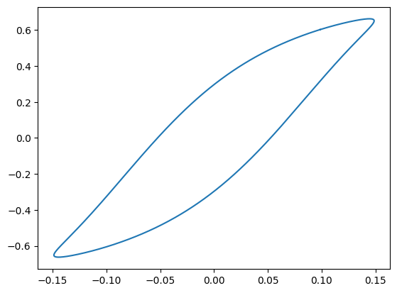

Now we generate random shapes to get a flavor of the variety of shapes that the parameterization can represent. Click the Generate Curve button below to initialize random $A$ matrices and visualize the resulting curves. The activation function used is LeakyReLU and it’s a 2 layer deep Injective Network.

Also, notice that the generated curve never self intersects.

Source

import numpy as np
import matplotlib.pyplot as plt
from ipywidgets import Button, VBox, Output, Layout
from IPython.display import display

def LeakyReLU(x, alpha = 0.1):
    return np.maximum(alpha * x, x)

def injective_net(t):
    # Perform the transformation for closed curves
    z = np.hstack([np.cos(2 * np.pi * t), np.sin(2 * np.pi * t)])
    a = LeakyReLU(z)

    # Perform the linear and non-linear transformations
    layer_count = 2
    for i in range(layer_count):
        A = np.random.random((2, 2)) - 0.5
        z = a @ A
        a = LeakyReLU(z)
    
    return a

# Create an output widget to display the plot
output = Output()

# Function to execute when the button is clicked
def generate_plot(_):
    with output:
        output.clear_output(wait = True)  # Clear previous output for fresh plot
        num_pts = 1000
        t = np.linspace(0, 1, num_pts).reshape(-1, 1)

        X = injective_net(t)

        # Plot the result
        plt.plot(X[:, 0], X[:, 1])
        plt.show()

# Create a button widget
button = Button(
    description = "Generate Curve",
)
button.on_click(generate_plot)

# Display the button and output together
display(VBox([button, output]))

Impossible Self-Intersection¶

We saw in Condition 1 - Simple Curves that the network will be injective with probability 1 if the weight matrices are generated at random with some given probability distribution over $2 \times 2$ matrices. But this does not mean that self-intersection is impossible, it is just extremely unlikely. It may happen during optimization when we change the network parameters that some of the weight matrices become non-invertible and may lead to self-intersecting shapes.

To make sure that self-intersection is actually impossible and not just unlikely we can first take the matrix exponential of the weight matrices in the network and then use them for the linear transformations. The matrix exponential is guaranteed to be invertible for any matrix and hence no matter what our weight matrix is (invertible or non-invertible) the matrix obtained after performing the matrix exponential will be invertible. This gives a hard guarantee on injectivity.

Mathematically at every linear layer with input $x$ and output $v$ ,

W \in \mathbb{R}^{2 \times 2} \\ A = e^{W} \\ v = Ax

(6)

where, $x$ denotes the current layers activations and $v$ represents the activations after the linear transformation is performed.

Fitting Target Curves: Curve Similarity Metrics¶

Now that we have a shape parameterization method that represents only simple closed curves, we would like to fit it to target shapes. This is useful in various scenarios: starting an optimization from a particular initial shape, exploring the representative power of a given depth network, the effect of activation functions on the types of shapes that we can represent etc.

Let’s say we have a target shape specified (say the Stanford Bunny^[3]) and we want our parameterization to represent that shape as closely as possible. To represent the given shape one way would be to tune the parameters of the representation scheme iteratively using a gradient descent optimization approach. This requires us to define an objective function that can then be optimized over. An appropriate objective for this task would be some measure of similarity(or dissimilarity) between the target curve and the one traced out by our parameterization. The objective function can then be maximized(or minimized) to fit the parameters.

For details on similarity metrics refer to the tutorial on Geometric Similarity Measures described on the webpage of geosimilarity, the geometric loss function library that we will use.

Here we will assume that we have some curve similarity measures available to us defined as loss functions in PyTorch. We will use these directly to fit shapes. In particular we have the following setup:

Table 1:The optimization problem setup

Object	Details
Shape Parameterization	Injective Net with parameters ϕ
Candidate Curve	Sampled at discrete $t \in [0, 1]$ from Injective Net, stored in $N_c\times 2$ matrix $X_c$
Target Curve	Specified curve to fit, stored in $N_t \times 2$ matrix $X_t$
Loss Function	$\mathcal{L}(X_t, X_c)$

Note that since $X_c$ is sampled from the network with parameters ϕ it is also a function of ϕ, $X_c = X_c(\phi)$ .

Goal: Use automatic differentiation to get gradients of the loss $\mathcal{L}(X_t, X_c)$ w.r.t. ϕ and then run gradient descent and tune the parameters.

Implementation¶

import torch
from torch import nn

class InjectiveNet(nn.Module):
    def __init__(self, layer_count, act_fn):
        super().__init__()

        # Define the transformation from t on the [0, 1] interval to unit circle
        self.closed_transform = lambda t: torch.hstack([
            torch.cos(2 * torch.pi * t),
            torch.sin(2 * torch.pi * t)
        ])

        layers = []
        for i in range(layer_count):
            layers.append(nn.Linear(2, 2))
            layers.append(act_fn())
        layers.append(nn.Linear(2, 2))
        
        self.linear_act_stack = nn.Sequential(*layers)
    
    def forward(self, t):
        x = self.closed_transform(t)
        x = self.linear_act_stack(x)
        return x

Now we train Injective Networks to fit target shapes. In particular we use loss functions from the geosimilarity python package. Refer to the geosimilarity web tutorial on API reference and available geometric loss functions. We use shapes from the shapes python module. We will use a circle and square as target shapes and the Mean Squared Error (MSE) loss function to quantify the difference between the parameterized and the target curve.

We also use the automate_training ^[4] function to hide the training details and focus on the parameterization. The plot_curve function plots the target and the parameterized curves and abstracts away the plotting details.

import geosimilarity as gs
from assets.shapes import circle, square
from assets.utils import automate_training, plot_curves

# Generate target curve points
num_pts = 1000
t = torch.linspace(0, 1, num_pts).reshape(-1, 1)
Xt_circle = circle(num_pts)
Xt_square = square(num_pts)

# Initialize networks to learn the target shapes and train
circle_net = InjectiveNet(layer_count = 3, act_fn = nn.Tanh)
square_net = InjectiveNet(layer_count = 3, act_fn = nn.Tanh)

print('Training Circle Net:')
automate_training(
    model = circle_net, loss_fn = gs.MSELoss(), X_train = t, Y_train = Xt_circle,
    learning_rate = 0.1, epochs = 1000, print_cost_every = 200
)
print('Training Square Net:')
automate_training(
    model = square_net, loss_fn = gs.MSELoss(), X_train = t, Y_train = Xt_square,
    learning_rate = 0.1, epochs = 1000, print_cost_every = 200
)

# Get final curve represented by the networks
Xc_circle = circle_net(t)
Xc_square = square_net(t)

# Plot the curves
plot_curves(Xc_circle, Xt_circle)
plot_curves(Xc_square, Xt_square)

Training Circle Net:
Epoch: [   1/1000]. Loss:    0.900208
Epoch: [ 200/1000]. Loss:    0.000204
Epoch: [ 400/1000]. Loss:    0.000073
Epoch: [ 600/1000]. Loss:    0.000045
Epoch: [ 800/1000]. Loss:    0.000038
Epoch: [1000/1000]. Loss:    0.000041
Training Square Net:
Epoch: [   1/1000]. Loss:    0.939890
Epoch: [ 200/1000]. Loss:    0.000862
Epoch: [ 400/1000]. Loss:    0.000329
Epoch: [ 600/1000]. Loss:    0.000242
Epoch: [ 800/1000]. Loss:    0.000198
Epoch: [1000/1000]. Loss:    0.000182

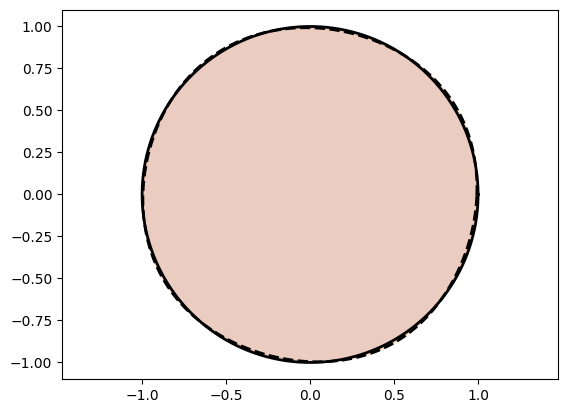
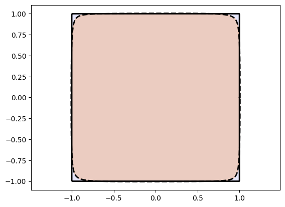
Awesome! We see that we are doing good on simple shapes.

Now we move onto something challenging.

Let’s test the method on the Stanford Bunny. We will treat the Stanford Bunny as our recurring evaluation target for different architectures. Therefore we will use a fixed number of points on the target bunny curve to maintain consistency across curve fitting results.

We now try different layer_count and act_fn to try and fit the bunny. We recommend you to play around with the code below to get a good feel for curve fitting capacity of Injective Networks.

from assets.shapes import stanford_bunny

# Generate target curve points
num_pts = 1000
t = torch.linspace(0, 1, num_pts).reshape(-1, 1)
Xt_bunny = stanford_bunny(num_pts)

bunny_net = InjectiveNet(layer_count = 4, act_fn = nn.Tanh)

automate_training(
    model = bunny_net, loss_fn = gs.MSELoss(), X_train = t, Y_train = Xt_bunny,
    learning_rate = 0.1, epochs = 1000, print_cost_every = 200
)

Xc_bunny = bunny_net(t)
plot_curves(Xc_bunny, Xt_bunny)

Epoch: [   1/1000]. Loss:    0.420288
Epoch: [ 200/1000]. Loss:    0.009758
Epoch: [ 400/1000]. Loss:    0.009648
Epoch: [ 600/1000]. Loss:    0.009597
Epoch: [ 800/1000]. Loss:    0.009503
Epoch: [1000/1000]. Loss:    0.009352

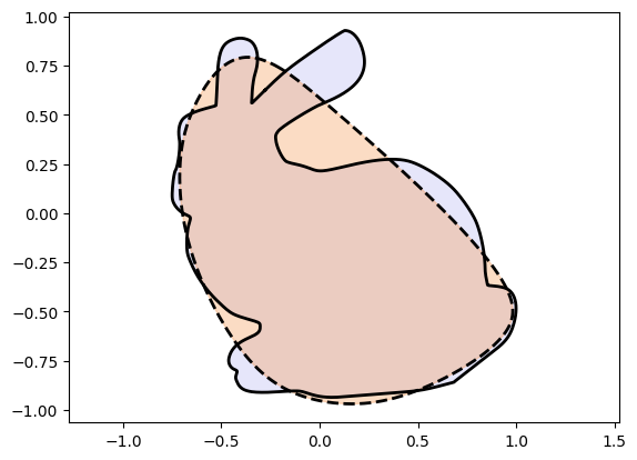
We observe very poor performance❗⚠️

If you played around with the code above you would have observed that Injective Networks on their own:

can get stuck in local optima.
can fail to be expressive enough.

To get ideas on improving the parameterization we first “cheat” a little and use the PReLU^[5] activation function. PReLU has a learnable slope parameter α which can during training become negative and therefore violate the injectivity property required from the activation function for non-self intersection. Therefore, in general PReLU cannot be used in Injective Networks but we use it here to gain insights into improving the method further.

from assets.shapes import stanford_bunny

# Generate target curve points
num_pts = 1000
t = torch.linspace(0, 1, num_pts).reshape(-1, 1)
Xt_bunny = stanford_bunny(num_pts)

bunny_net = InjectiveNet(layer_count = 5, act_fn = nn.PReLU)

automate_training(
    model = bunny_net, loss_fn = gs.MSELoss(), X_train = t, Y_train = Xt_bunny,
    learning_rate = 0.1, epochs = 1000, print_cost_every = 200
)

Xc_bunny = bunny_net(t)
plot_curves(Xc_bunny, Xt_bunny)

Epoch: [   1/1000]. Loss:    0.577817
Epoch: [ 200/1000]. Loss:    0.161443
Epoch: [ 400/1000]. Loss:    0.003423
Epoch: [ 600/1000]. Loss:    0.002988
Epoch: [ 800/1000]. Loss:    0.005976
Epoch: [1000/1000]. Loss:    0.002146

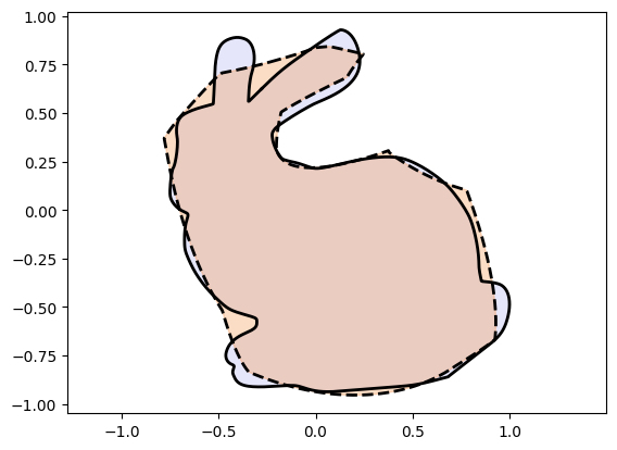
We see an exciting improvement! Injective Networks with PReLU do much better. This gives us the following insight:

Injective Networks are parameter deficient.

Adding parameters gives them much more representation power.

We now address this problem of parameter deficiency and solve it using Monotonic Networks.

Footnotes¶

A square $n \times n$ matrix is injective if and only if it is invertible.
Singular matrices are rare in the sense that if a square matrix’s entries are randomly selected from any bounded region on the number line or complex plane, the probability that the matrix is singular is 0, that is, it will “almost never” be singular.
Wikipedia, Invertible Matrix
↩
Composition of two injective functions $f$ and $g$ , $f \circ g$ is also injective. Wikipedia, Injective function
↩
The Stanford Bunny
The Stanford Bunny. We will use it as a target shape against which we test our parameterization techniques.
↩

The code used for automating the training of Networks is:

utils.py

def automate_training(
        model,
        loss_fn,
        X_train: torch.Tensor,
        Y_train: torch.Tensor,
        epochs: int = 1000,
        print_cost_every: int = 200,
        learning_rate: float = 0.001,
) -> None:
    optimizer = torch.optim.Adam(model.parameters(), lr = learning_rate)
    scheduler = torch.optim.lr_scheduler.ReduceLROnPlateau(optimizer, factor = 0.99)

    for epoch in range(epochs):
        Y_model = model(X_train)
        loss = loss_fn(Y_model, Y_train)

        loss.backward()
        optimizer.step()
        optimizer.zero_grad()
        scheduler.step(loss.item())

        if epoch == 0 or (epoch + 1) % print_cost_every == 0:
            num_digits = len(str(epochs))
            print(f'Epoch: [{epoch + 1:{num_digits}}/{epochs}]. Loss: {loss.item():11.6f}')

↩

PyTorch PReLU
Applies the element-wise PReLU function.
$\text{PReLU}(x) = \max(0,x) + a * \min(0,x)$
(7)
or
$\text{PReLU}(x) = \begin{cases} x, & \text{ if } x \ge 0 \\ ax, & \text{ otherwise } \end{cases}$
(8)
Here $a$ is a learnable parameter. When called without arguments, nn.PReLU() uses a single parameter $a$ across all input channels.
↩

Neural Injective Geometry

Motivation for Non-Self-Intersecting Geometry

Injective Networks

Injective Networks Showcase