We now fit Injective Networks to some target shapes to get a sense of their representation power and shortcomings.
# Basic imports
import torch
from torch import nn
import geosimilarity as gs
from NIGnets import NIGnet

from assets.utils import automate_training, plot_curves
We will now start using the NIGnets package for creating networks instead of defining them again and again with additional features.
Intersection Possible
We now fit Injective Networks to target curves when there are no additional constraints on the network weight matrices and therefore, non-invertibility of weight matrices is possible during optimization.
Circle and Square
from assets.shapes import circle, square

# Generate target curve points
num_pts = 1000
t = torch.linspace(0, 1, num_pts).reshape(-1, 1)
Xt_circle = circle(num_pts)
Xt_square = square(num_pts)

# Initialize networks to learn the target shapes and train
circle_net = NIGnet(layer_count = 3, act_fn = nn.Tanh)
square_net = NIGnet(layer_count = 3, act_fn = nn.Tanh)

print('Training Circle Net:')
automate_training(
    model = circle_net, loss_fn = gs.MSELoss(), X_train = t, Y_train = Xt_circle,
    learning_rate = 0.1, epochs = 1000, print_cost_every = 200
)
print('Training Square Net:')
automate_training(
    model = square_net, loss_fn = gs.MSELoss(), X_train = t, Y_train = Xt_square,
    learning_rate = 0.1, epochs = 1000, print_cost_every = 200
)

# Get final curve represented by the networks
Xc_circle = circle_net(t)
Xc_square = square_net(t)

# Plot the curves
plot_curves(Xc_circle, Xt_circle)
plot_curves(Xc_square, Xt_square)
Training Circle Net:
Epoch: [ 1/1000]. Loss: 0.633713
Epoch: [ 200/1000]. Loss: 0.000025
Epoch: [ 400/1000]. Loss: 0.000011
Epoch: [ 600/1000]. Loss: 0.000008
Epoch: [ 800/1000]. Loss: 0.000006
Epoch: [1000/1000]. Loss: 0.000004
Training Square Net:
Epoch: [ 1/1000]. Loss: 0.898328
Epoch: [ 200/1000]. Loss: 0.001820
Epoch: [ 400/1000]. Loss: 0.000804
Epoch: [ 600/1000]. Loss: 0.000731
Epoch: [ 800/1000]. Loss: 0.000710
Epoch: [1000/1000]. Loss: 0.000704
Stanford Bunny
from assets.shapes import stanford_bunny

# Generate target curve points
num_pts = 1000
t = torch.linspace(0, 1, num_pts).reshape(-1, 1)
Xt_bunny = stanford_bunny(num_pts)

bunny_net = NIGnet(layer_count = 5, act_fn = nn.Tanh)

automate_training(
    model = bunny_net, loss_fn = gs.MSELoss(), X_train = t, Y_train = Xt_bunny,
    learning_rate = 0.1, epochs = 1000, print_cost_every = 200
)

Xc_bunny = bunny_net(t)
plot_curves(Xc_bunny, Xt_bunny)
Epoch: [ 1/1000]. Loss: 0.386537
Epoch: [ 200/1000]. Loss: 0.017831
Epoch: [ 400/1000]. Loss: 0.005423
Epoch: [ 600/1000]. Loss: 0.004649
Epoch: [ 800/1000]. Loss: 0.004336
Epoch: [1000/1000]. Loss: 0.004233
Airfoil
from assets.shapes import airfoil

# Generate target curve points
num_pts = 1000
t = torch.linspace(0, 1, num_pts).reshape(-1, 1)
Xt_airfoil = airfoil(num_pts)

airfoil_net = NIGnet(layer_count = 4, act_fn = nn.Tanh)

automate_training(
    model = airfoil_net, loss_fn = gs.MSELoss(), X_train = t, Y_train = Xt_airfoil,
    learning_rate = 0.1, epochs = 1000, print_cost_every = 200
)

Xc_airfoil = airfoil_net(t)
plot_curves(Xc_airfoil, Xt_airfoil)
Epoch: [ 1/1000]. Loss: 0.289349
Epoch: [ 200/1000]. Loss: 0.000710
Epoch: [ 400/1000]. Loss: 0.000083
Epoch: [ 600/1000]. Loss: 0.000057
Epoch: [ 800/1000]. Loss: 0.000046
Epoch: [1000/1000]. Loss: 0.000040
Intersection Impossible
We now fit Injective Networks to target curves when we first perform a matrix exponential of the weight matrices and then use them for the linear transformations. Therefore, non-invertibility of weight matrices is impossible during optimization.
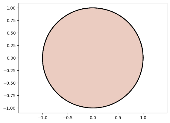
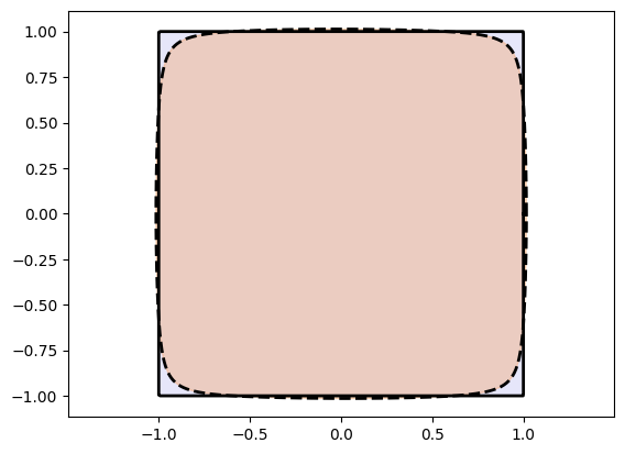
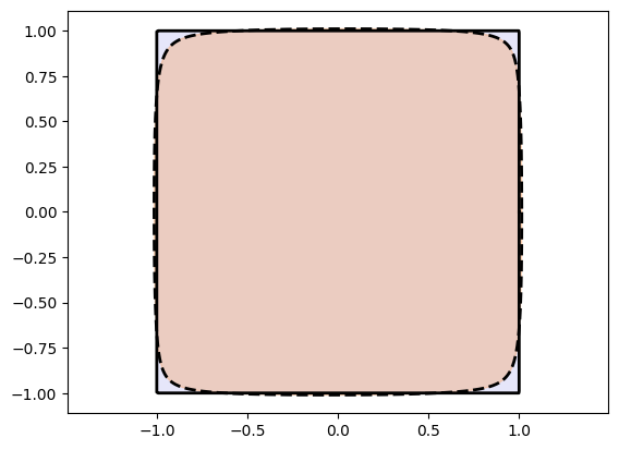
Circle and Square
from assets.shapes import circle, square

# Generate target curve points
num_pts = 1000
t = torch.linspace(0, 1, num_pts).reshape(-1, 1)
Xt_circle = circle(num_pts)
Xt_square = square(num_pts)

# Initialize networks to learn the target shapes and train
circle_net = NIGnet(layer_count = 3, act_fn = nn.Tanh, intersection = 'impossible')
square_net = NIGnet(layer_count = 3, act_fn = nn.Tanh, intersection = 'impossible')

print('Training Circle Net:')
automate_training(
    model = circle_net, loss_fn = gs.MSELoss(), X_train = t, Y_train = Xt_circle,
    learning_rate = 0.1, epochs = 1000, print_cost_every = 200
)
print('Training Square Net:')
automate_training(
    model = square_net, loss_fn = gs.MSELoss(), X_train = t, Y_train = Xt_square,
    learning_rate = 0.1, epochs = 1000, print_cost_every = 200
)

# Get final curve represented by the networks
Xc_circle = circle_net(t)
Xc_square = square_net(t)

# Plot the curves
plot_curves(Xc_circle, Xt_circle)
plot_curves(Xc_square, Xt_square)
Training Circle Net:
Epoch: [ 1/1000]. Loss: 0.365332
Epoch: [ 200/1000]. Loss: 0.001869
Epoch: [ 400/1000]. Loss: 0.000162
Epoch: [ 600/1000]. Loss: 0.002354
Epoch: [ 800/1000]. Loss: 0.000030
Epoch: [1000/1000]. Loss: 0.000030
Training Square Net:
Epoch: [ 1/1000]. Loss: 0.495981
Epoch: [ 200/1000]. Loss: 0.000615
Epoch: [ 400/1000]. Loss: 0.000589
Epoch: [ 600/1000]. Loss: 0.000577
Epoch: [ 800/1000]. Loss: 0.000545
Epoch: [1000/1000]. Loss: 0.000708

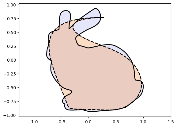
Stanford Bunny
from assets.shapes import stanford_bunny

# Generate target curve points
num_pts = 1000
t = torch.linspace(0, 1, num_pts).reshape(-1, 1)
Xt_bunny = stanford_bunny(num_pts)

bunny_net = NIGnet(layer_count = 5, act_fn = nn.Tanh, intersection = 'impossible')

automate_training(
    model = bunny_net, loss_fn = gs.MSELoss(), X_train = t, Y_train = Xt_bunny,
    learning_rate = 0.1, epochs = 1000, print_cost_every = 200
)

Xc_bunny = bunny_net(t)
plot_curves(Xc_bunny, Xt_bunny)
Epoch: [ 1/1000]. Loss: 1.172325
Epoch: [ 200/1000]. Loss: 0.029859
Epoch: [ 400/1000]. Loss: 0.030550
Epoch: [ 600/1000]. Loss: 0.020915
Epoch: [ 800/1000]. Loss: 0.022760
Epoch: [1000/1000]. Loss: 0.019492
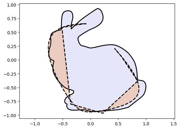
Above we include a pathological fit to drive the following point:
num_pts = 10000
t = torch.linspace(0, 1, num_pts).reshape(-1, 1)
Xt_bunny = stanford_bunny(num_pts)

Xc_bunny = bunny_net(t)
plot_curves(Xc_bunny, Xt_bunny)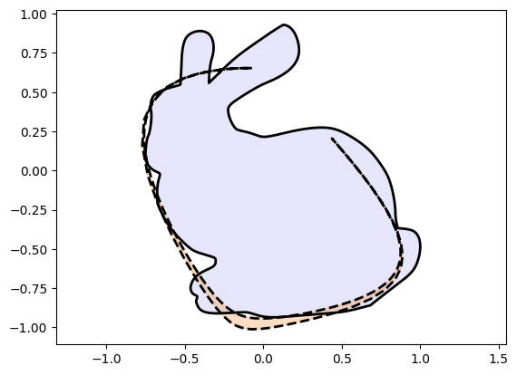
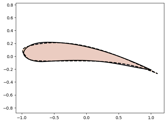
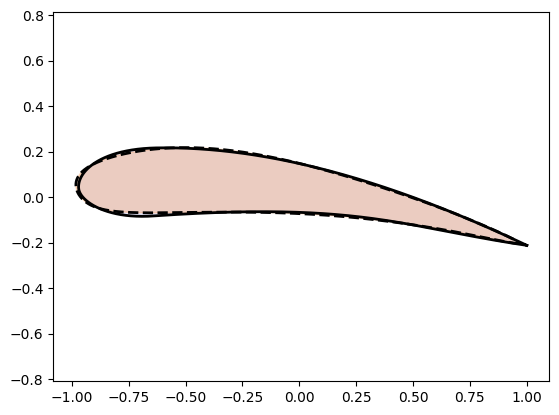
Airfoil
from assets.shapes import airfoil

# Generate target curve points
num_pts = 1000
t = torch.linspace(0, 1, num_pts).reshape(-1, 1)
Xt_airfoil = airfoil(num_pts)

airfoil_net = NIGnet(layer_count = 4, act_fn = nn.Tanh, intersection = 'impossible')

automate_training(
    model = airfoil_net, loss_fn = gs.USDFLoss(), X_train = t, Y_train = Xt_airfoil,
    learning_rate = 0.01, epochs = 1000, print_cost_every = 200
)

Xc_airfoil = airfoil_net(t)
plot_curves(Xc_airfoil, Xt_airfoil)
Epoch: [ 1/1000]. Loss: 0.104689
Epoch: [ 200/1000]. Loss: 0.001453
Epoch: [ 400/1000]. Loss: 0.000817
Epoch: [ 600/1000]. Loss: 0.000388
Epoch: [ 800/1000]. Loss: 0.000117
Epoch: [1000/1000]. Loss: 0.000094