Monotonic Networks

Creating Injective Functions with Parameters¶

We observed earlier that with the PReLU activation Injective Networks perform much better. Therefore, the insight we gain that will help us power up Injective Networks is : add more parameters.

One way to add parameters to the Network is to use parameterized activation functions e.g. $\sigma(\beta x)$ i.e. the sigmoid with a parameter β or try and create other activations. During the creation of these parameterized activations one needs to keep in mind that injectivity should not be violated for any parameter value to ensure that the network always represents only simple closed curves, which is our final goal.

It is quite difficult to combine activation functions together with appropriate parameters that add representation power while maintaining injectivity. We will therefore look at a much more drastic and interesting approach.

First, we need to understand how we could create a function that is injective. The first step is to realize that:

A continuous function is injective if and only if it is strictly monotonic.^[1]

Therefore we can create injective functions by creating strictly monotonic functions.

Monotonic Networks: A Superpower¶

We will create injective activation functions using a drastic measure. Every activation function will be an injective neural network!

We will create neural networks that take in a scalar input and output a scalar value and are strictly monotonic in the input. Mathematically our activation function now is a neural network $M$

which satisfies one of:

Every activation layer will be an independent Monotonic Network and all neurons will use the same neural network. This is shown in Figure 1.

Building Monotonic Networks with Smooth Min-Max Networks¶

Building Monotonic Networks is an active area of research and there are a few popular choices. The first Monotonic Network was designed by Sill (1997) which used $min$ and $max$ operations to impart monotonicity. But since the $min-max$ operations are not differentiable they are hard to train and also suffer from dead neurons^[2]. Recently Igel (2023) proposed a variation of the original Monotonic Networks proposed by Sill (1997), which replaces the hard $min-max$ with their smooth variants. These are called Smooth Min-Max Monotonic Networks.

We will use Smooth Min-Max Monotonic Networks as activation functions to augment Injective Networks. We use the code provided in Christian’s Repository https://github.com/christian-igel/SMM as reference for our own code.

Note: To ensure positive weights for monotonicity constraints we provide two options.

• Exponential positivity: $w = e^z$ - Igel (2023) and Sill (1997)
• Squared positivity: $w = z^2$ - Daniels & Velikova (2010)

By default monotonic networks provided in the NIGnets module use squared positivity constraints as they were found to perform slightly better.

To use monotonic networks with NIGnets, create a monotonic network of a particular architecture and pass that as an input to NIGnets. NIGnets under the hood creates deepcopies using the same architecture and uses different monotonic networks at each layer. The NIGnets package comes with an implementation of some popular monotonic networks that can be used directly without installing additional dependencies.

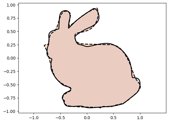
We observe an amazing improvement! Using Monotonic Networks as activation functions bolsters Injective Networks by introducing a lot of parameters which can be tuned to fit shapes with high accuracy.

Skip Connections: ResNet Style¶

The Residual Network (ResNet) architecture has made training easier for deeper networks. We can similarly use skip connections with monotonic networks as they preserve monotonicity and hence injectivity. This will allow us to train deeper NIGnets. The skip connection connects the input with the output of a subnetwork. This is shown in Figure 2.

We now see that we can have skip connections after each layer in NIGnets and still maintain injectivity of the layers separately and therefore of the network as a whole.

Linear Layers

Each linear layer performs the operation $y = Ax$. Adding a skip connection would lead to:

$$y = Ax + x = (A + I)x$$

(3)

A skip connection is mathematically unnecessary in a mathematical sense as we can think of any transformation $Ax$ to be composed of $(B + I)x$ and view $B$ as our weight matrix for the layer instead. In fact using skip connections with the Impossible Self-Intersection can lead to non-invertible matrices and violate the hard guarantee on injectivity. This is because even though $e^{A}$ is always invertible, $e^{A} + I$ is not and may even be the 0 matrix. Thus, we do not use skip connections with the linear layer.

Nonlinear Layers

For the nonlinear transformations we use some injective scalar-valued mapping, which is either an activation function or a monotonic network. Assuming that the mapping is an increasing monotonic function $M(x)$. Then we have the layer’s transformation $L(x)$ to be:

$$L(x) = M(x) + x$$

(4)

Taking derivative,

$$L'(x) = M'(x) + 1$$

(5)

now since $M(x)$ is an increasing monotonic function, $M'(x)$ is positive and hence we also have,

$$L'(x) >= 1$$

(6)

Thus the resulting transformation is also an increasing monotonic function. The derivative being always greater than 1, might be a concern and we could additionally also include a positively constrained scaling to $x$ as:

$$L(x) = M(x) + \alpha x$$

(7)

with,

$$L'(x) = M'(x) + \alpha >= 0$$

(8)

NIGnets uses a squared positivity constraint and uses the scaling $\alpha^2 x$ with α being the parameter.

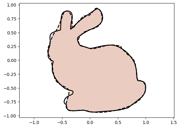
Training dynamics and performance with skip connections we find to be so good that NIGnets by default uses skip connections. To not use skip connections pass in the additional argument skip_connections = False to the NIGnet constructor.