We now fit 3D NIGnets to some target shapes to get a sense of their representation power and shortcomings.
# Basic imports
import torch
from torch import nn
import geosimilarity as gs
from NIGnets import NIGnet
from NIGnets.monotonic_nets import SmoothMinMaxNet

from assets.utils import automate_training, plot_surfaces

device = 'mps' if torch.backends.mps.is_available() else 'cpu'
We will use the following network architecture for PreAux nets in this showcase. Users need to define their own PreAux net architectures similarly making sure that the conditions on the output are met Paragraph.
class PreAuxNet(nn.Module):
def __init__(self, layer_count, hidden_dim):
super().__init__()
# Pre-Auxilliary net needs closed transform to get same r at theta = 0, 2pi
self.closed_transform = lambda t, s: torch.hstack([
torch.sin(torch.pi * s) * torch.cos(2 * torch.pi * t),
torch.sin(torch.pi * s) * torch.sin(2 * torch.pi * t),
torch.cos(torch.pi * s)
])
layers = [nn.Linear(3, hidden_dim), nn.BatchNorm1d(hidden_dim), nn.PReLU()]
for i in range(layer_count):
layers.append(nn.Linear(hidden_dim, hidden_dim))
layers.append(nn.BatchNorm1d(hidden_dim))
layers.append(nn.PReLU())
layers.append(nn.Linear(hidden_dim, 1))
layers.append(nn.ReLU())
self.forward_stack = nn.Sequential(*layers)
def forward(self, t, s):
unit_sphere = self.closed_transform(t, s)
r = self.forward_stack(unit_sphere)
X = r * unit_sphere
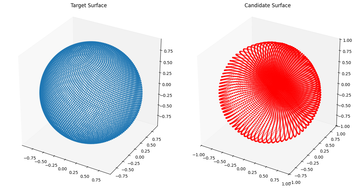
return XSphere and Cube
from assets.shapes import sphere

# Generate target curve points
num_pts = 100
t, s = torch.meshgrid(torch.linspace(0, 1, num_pts), torch.linspace(0, 1, num_pts),
                      indexing = 'ij')
T = torch.stack([t, s], dim = -1).reshape(-1, 2).to(device)
Xt = sphere(num_pts * num_pts).to(device)

# Create NIGnet to fit the target
preaux_net = PreAuxNet(layer_count = 2, hidden_dim = 15)
monotonic_net = SmoothMinMaxNet(input_dim = 1, n_groups = 3, nodes_per_group = 3)
nig_net = NIGnet(layer_count = 3, preaux_net = preaux_net, monotonic_net = monotonic_net,
                 geometry_dim = 3, skip_connections = False).to(device)

automate_training(
    model = nig_net, loss_fn = gs.ChamferLoss(), X_train = T, Y_train = Xt,
    learning_rate = 0.1, epochs = 1000, print_cost_every = 200
)

# Plot the candidate and the target geometries
Xc = nig_net(T)
plot_surfaces(Xc, Xt)
Epoch: [ 1/1000]. Loss: 1.505007
Epoch: [ 200/1000]. Loss: 0.000960
Epoch: [ 400/1000]. Loss: 0.000690
Epoch: [ 600/1000]. Loss: 0.002493
Epoch: [ 800/1000]. Loss: 0.000633
Epoch: [1000/1000]. Loss: 0.000622
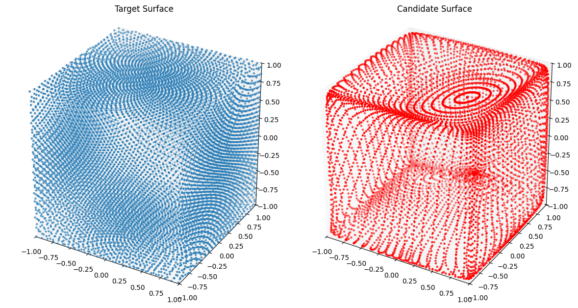
from assets.shapes import cube

# Generate target curve points
num_pts = 100
t, s = torch.meshgrid(torch.linspace(0, 1, num_pts), torch.linspace(0, 1, num_pts),
                      indexing = 'ij')
T = torch.stack([t, s], dim = -1).reshape(-1, 2).to(device)
Xt = cube(num_pts * num_pts).to(device)

# Create NIGnet to fit the target
preaux_net = PreAuxNet(layer_count = 2, hidden_dim = 15)
monotonic_net = SmoothMinMaxNet(input_dim = 1, n_groups = 5, nodes_per_group = 5)
nig_net = NIGnet(layer_count = 3, preaux_net = preaux_net, monotonic_net = monotonic_net,
                 geometry_dim = 3, skip_connections = False).to(device)

automate_training(
    model = nig_net, loss_fn = gs.ChamferLoss(), X_train = T, Y_train = Xt,
    learning_rate = 0.1, epochs = 1000, print_cost_every = 200
)

# Plot the candidate and the target geometries
Xc = nig_net(T)
plot_surfaces(Xc, Xt)
Epoch: [ 1/1000]. Loss: 2.127341
Epoch: [ 200/1000]. Loss: 0.004418
Epoch: [ 400/1000]. Loss: 0.002507
Epoch: [ 600/1000]. Loss: 0.001962
Epoch: [ 800/1000]. Loss: 0.001924
Epoch: [1000/1000]. Loss: 0.002003
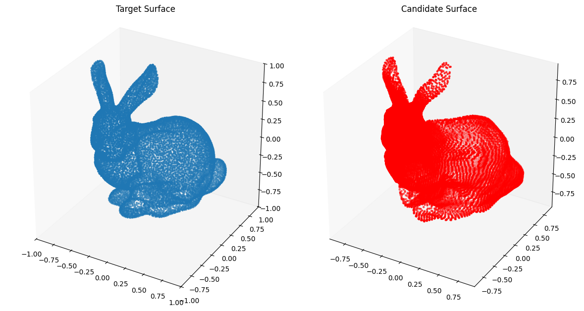
Stanford Bunny
from assets.shapes import stanford_bunny_3d

# Generate target curve points
num_pts = 100
t, s = torch.meshgrid(torch.linspace(0, 1, num_pts), torch.linspace(0, 1, num_pts),
                      indexing = 'ij')
T = torch.stack([t, s], dim = -1).reshape(-1, 2).to(device)
Xt = stanford_bunny_3d(num_pts * num_pts).to(device)

# Create NIGnet to fit the target
preaux_net = PreAuxNet(layer_count = 5, hidden_dim = 100)
monotonic_net = SmoothMinMaxNet(input_dim = 1, n_groups = 15, nodes_per_group = 15)
nig_net = NIGnet(layer_count = 5, preaux_net = preaux_net, monotonic_net = monotonic_net,
                 geometry_dim = 3).to(device)

automate_training(
    model = nig_net, loss_fn = gs.ChamferLoss(), X_train = T, Y_train = Xt,
    learning_rate = 0.1, epochs = 10000, print_cost_every = 2000
)

# Plot the candidate and the target geometries
Xc = nig_net(T)
plot_surfaces(Xc, Xt)
Epoch: [ 1/10000]. Loss: 1.014258
Epoch: [ 2000/10000]. Loss: 0.001180
Epoch: [ 4000/10000]. Loss: 0.000678
Epoch: [ 6000/10000]. Loss: 0.000590
Epoch: [ 8000/10000]. Loss: 0.000575
Epoch: [10000/10000]. Loss: 0.000572
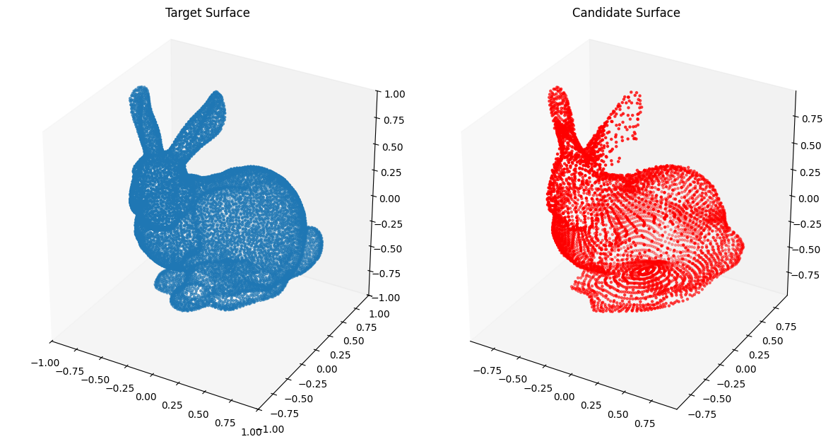
The closed transform from the unit square to the unit sphere as we did earlier leads to concentration of points on the poles of the sphere. Therefore, we try using a closed transform that distributes the points uniformly on the surface of the sphere.
def sphere_from_t(num_pts: int) -> torch.Tensor:
    """Generates approximately evenly distributed points on the unit sphere using the Fibonacci
    lattice.
    """
    idx = torch.arange(0, num_pts) + 0.5
    phi = torch.arccos(1 - 2 * idx / num_pts)
    theta = torch.pi * (1 + 5**0.5) * idx

    # Compute x, y and z coordinates
    x = torch.sin(phi) * torch.cos(theta)
    y = torch.sin(phi) * torch.sin(theta)
    z = torch.cos(phi)

    # Concatenate to form a matrix of shape: (num_pts, 3)
    X = torch.stack([x, y, z], dim = 1)
    return X

class PreAuxNet(nn.Module):
    def __init__(self, layer_count, hidden_dim):
        super().__init__()

        # Pre-Auxilliary net needs closed transform to get same r at theta = 0, 2pi
        self.closed_transform = sphere_from_t

        layers = [nn.Linear(3, hidden_dim), nn.BatchNorm1d(hidden_dim), nn.PReLU()]
        for i in range(layer_count):
            layers.append(nn.Linear(hidden_dim, hidden_dim))
            layers.append(nn.BatchNorm1d(hidden_dim))
            layers.append(nn.PReLU())
        layers.append(nn.Linear(hidden_dim, 1))
        layers.append(nn.ReLU())

        self.forward_stack = nn.Sequential(*layers)

    def forward(self, t, s):
        unit_sphere = self.closed_transform(t.shape[0]).to('mps')

        r = self.forward_stack(unit_sphere)
        X = r * unit_sphere
        return X
from assets.shapes import stanford_bunny_3d
# Generate target curve points
num_pts = 200
t, s = torch.meshgrid(torch.linspace(0, 1, num_pts), torch.linspace(0, 1, num_pts),
indexing = 'ij')
T = torch.stack([t, s], dim = -1).reshape(-1, 2).to(device)
Xt = stanford_bunny_3d(num_pts * num_pts // 4).to(device)
# Create NIGnet to fit the target
preaux_net = PreAuxNet(layer_count = 5, hidden_dim = 100)
monotonic_net = SmoothMinMaxNet(input_dim = 1, n_groups = 15, nodes_per_group = 15)
nig_net = NIGnet(layer_count = 5, preaux_net = preaux_net, monotonic_net = monotonic_net,
geometry_dim = 3).to(device)
automate_training(
model = nig_net, loss_fn = gs.ChamferLoss(), X_train = T, Y_train = Xt,
learning_rate = 0.1, epochs = 1000, print_cost_every = 200
)
# Plot the candidate and the target geometries
Xc = nig_net(T)
plot_surfaces(Xc, Xt)