CST - Class Shape Transformation

Class Shape Transformation (CST) is a classical approach popularly used for parameterizing airfoil and wing shapes though it is quite general and can also be used to represent other aircraft components. It uses class functions and shape functions to parameterize shapes. The class function decides the family of shapes and the shape function provides expressivity to fit different shapes within that class and also the ability to directly control key geometry parameters such as leading edge radius, trailing edge boattail angle, and closure to a specified aft thickness. In this tutorial, we walk through the theory behind the CST representation and how to actually use their geodiff implementation in practice.

# Basic Imports
import matplotlib.pyplot as plt
import torch

from geodiff.cst import CST
from geodiff.loss_functions.chamfer import ChamferLoss

from assets.utils import square, normalize_0_to_1

Theoretical Background¶

The CST representation works by combining class functions and shape functions. The shape is represented by the following equations Kulfan & Bussoletti, 2006:

\begin{align*} y_u(x) &= C(x) \, S_u(x) + \Delta y_{u} \\ y_l(x) &= C(x) \, S_l(x) - \Delta y_{l} \end{align*}

(1)

where, $x \in [0, 1]$ . $y_{u}$ and $y_{l}$ are the ordinates of the upper and lower surfaces of the geometry. $C(x)$ is the class function:

C(x) = x^{n_1} \left(1 - x \right)^{n_2}

(2)

specified by exponents $n_1$ and $n_2$ . $S_u(x)$ and $S_l(x)$ are the shape functions for the upper and lower surfaces described by:

S_u(x) = \sum_{k=0}^{K_u} A_{u,k} \, S_k(x), \qquad S_l(x) = \sum_{k=0}^{K_l} A_{l,k} \, S_k(x)

(3)

where the element shape functions $S_k(x)$ are the Bernstein basis polynomials ^[1] of degree $K$ :

S_k(x) = \binom{K}{k} x^{k} (1 - x)^{K - k}, \qquad \text{for} \; k = 0, \ldots, K

(4)

$\Delta y_{u}$ and $\Delta y_{l}$ are trailing-edge offsets that govern the trailing-edge thickness, specifically:

t_{TE} = \Delta y_{u} + \Delta y_{l}

(5)

Note that, we define both quantities to be positive always, this allows us to compute the thickness at the trailing edge simply as $y_{u} - y_{l}$ since the class function at $x = 1$ vanishes.

Implementation using `geodiff`¶

We now look at how geodiff allows us to easily use the CST parameterization to represent shapes.

The CST class initializer and its expected arguments are shown below:

cst.py

    def __init__(
        self,
        n1: float = 0.5,
        n2: float = 1.0,
        upper_basis_count: int = 9,
        lower_basis_count: int = 9,
        upper_te_thickness: float = 0.0,
        lower_te_thickness: float = 0.0,
    ) -> None:

To construct a CST object, we may supply:

Class function exponents n_1 and n_2.
Shape function basis count for the upper and lower surfaces. The degree of the Bernstein polynomial used will be one less than the basis count.
Trailing edge thicknesses for the upper and lower surfaces.

Fitting Shapes¶

We will use a square as our target geometry. We then use the ChamferLoss to compute the geometric difference loss between the target shape and the shape represented by our CST parameterization. Since the implementation is written in PyTorch we can use the autograd capabilities to compute the gradients of the loss w.r.t. the CST shape function coefficients and use an optimizer to modify our geometry.

We start by obtaining points on our shapes and normalizing them appropriately such that $x \in [0, 1]$ as assumed by the implementation.

# Get points on a square (curve to fit)
num_pts = 1000
X_square = square(num_pts)

# For CST x values should lie in the range [0, 1]
X_square = normalize_0_to_1(X_square)

We now create a CST object by specifying the class function exponents, the basis function counts and the trailing edge thicknesses.

# Create a CST object
cst = CST(
    n1 = 0.5,
    n2 = 0.5,
    upper_basis_count = 12,
    lower_basis_count = 12,
    upper_te_thickness = 0,
    lower_te_thickness = 0
)

We use the ChamferLoss provided by geodiff to compute a geometric loss between the target shape and the shape represented by the CST object. PyTorch’s autograd capabilities then allow us to compute gradients of the loss w.r.t. the CST shape function coefficients and modify them to fit the target shape.

# Train the CST parameters to fit the square
loss_fn = ChamferLoss()

learning_rate = 0.001
epochs = 1000
print_cost_every = 200

Y_train = X_square

optimizer = torch.optim.Adam(cst.parameters(), lr = learning_rate)
scheduler = torch.optim.lr_scheduler.ReduceLROnPlateau(optimizer, factor = 0.99)

for epoch in range(epochs):
    Y_model = cst(num_pts = num_pts)
    Y_model = torch.vstack([Y_model[0], Y_model[1]])
    
    loss = loss_fn(Y_model, Y_train)

    loss.backward()
    optimizer.step()
    optimizer.zero_grad()
    scheduler.step(loss.item())

    if epoch == 0 or (epoch + 1) % print_cost_every == 0:
        num_digits = len(str(epochs))
        print(f'Epoch: [{epoch + 1:{num_digits}}/{epochs}]. Loss: {loss.item():11.6f}')

Epoch: [   1/1000]. Loss:    0.012038
Epoch: [ 200/1000]. Loss:    0.006183
Epoch: [ 400/1000]. Loss:    0.003808
Epoch: [ 600/1000]. Loss:    0.002843
Epoch: [ 800/1000]. Loss:    0.002256
Epoch: [1000/1000]. Loss:    0.001787

We can now visualize the shape represented by our CST object using its visualize method.

# Visualize the fitted CST shape
fig, ax = cst.visualize(num_pts = num_pts)
plt.tight_layout()
plt.show()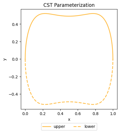

Footnotes¶

Bernstein basis polynomials are basis functions that form a partition of unity. The $n + 1$ Bernstein basis polynomials of degree $n$ are defined as:
$b_{k, n}(x) = \binom{n}{k} x^{k} (1 - x)^{n - k}, \qquad \text{for} \; k = 0, \ldots, n$
(6)
where $\binom{n}{k}$ is a binomial coefficient.
Wikipedia, Bernstein Polynomial
↩

References¶

Kulfan, B., & Bussoletti, J. (2006). “ Fundamental” parameteric geometry representations for aircraft component shapes. 11th AIAA/ISSMO Multidisciplinary Analysis and Optimization Conference, 6948.

GeoDiff

Hicks-Henne Bump Functions

GeoDiff

NICE - Nonlinear Independent Components Estimation

CST - Class Shape Transformation

Theoretical Background¶

Implementation using geodiff¶

Fitting Shapes¶

Implementation using `geodiff`¶