Hicks-Henne Bump Functions

Hicks-Henne bump function representation is a classical approach for parameterizing airfoil and wing shapes. It uses two families of bump functions^[1], which are added linearly onto a baseline geometry to produce a modified shape. In this tutorial, we walk through the theory behind Hicks-Henne bump functions and how to actually use their geodiff implementation in practice.

History behind the Hicks-Henne bump functions

The Hicks-Henne bump function parameterization was popularized by the paper titled “Wing design by numerical optimization” Hicks & Henne, 1978. Almost all references to the Hicks-Henne parameterization point to this paper. But, this paper does not list the functional form of the Hicks-Henne basis functions. These were introduced in a prior paper “Application of Numerical Optimization to the Design of Supercritical Airfoils without Drag-Creep.” Hicks & Vanderplaats, 1977. So the actual basis functions were used by Hicks and Vanderplaats but the name Hicks-Henne has stuck since their paper popularized it.

# Basic Imports
import matplotlib.pyplot as plt
import torch

from geodiff.hicks_henne import HicksHenne
from geodiff.loss_functions.chamfer import ChamferLoss

from assets.utils import circle, square, normalize_0_to_1

Theoretical Background¶

Hicks-Henne representation works by modifying a baseline geometry. The shape is represented by the following equations Hicks & Henne, 1978:

y_{upper} = y_{upper}^{baseline} + \sum_i a_i f_i \\[2ex] y_{lower} = y_{lower}^{baseline} + \sum_i b_i g_i

(1)

where, $y_{upper}^{baseline}$ and $y_{lower}^{baseline}$ are the ordinates of the upper and lower surfaces of the baseline geometry, and $f_i$ and $g_i$ are basis functions that are added linearly to modify the shape. The contribution of each function is determined by the value of the participation coefficients (design variables), $a_i$ s and $b_i$ s, associated with that function. All participation coefficients are initially set to zero to represent the baseline geometry.

Two classes of basis functions are used: 1) polynomial-exponential and 2) sinusoidal. The functional forms of these are defined in Eq. (2) and Eq. (3) respectively Hicks & Vanderplaats, 1977.

y = \frac{\left(x \right)^{n} \left(1 - x \right)}{e^{mx}}

(2)

y = \sin \left( \pi x^{n} \right)^{m}

(3)

where, $x \in [0, 1]$ .

Graphs of these functions for various values of $n$ and $m$ are shown in Figure 1 and Figure 2^[2]. Note that the region of influence of the functions is controlled by the exponents $n$ and $m$ . The chordwise location of the peak of the sine curves in Eq. (3) is proportional to the exponent $n$ , whereas the width of each curve is determined by $m$ Figure 1. The location and magnitude of the peak of the polynomial- exponential functions in Eq. (2) are determined by both $n$ and $m$ Figure 2.

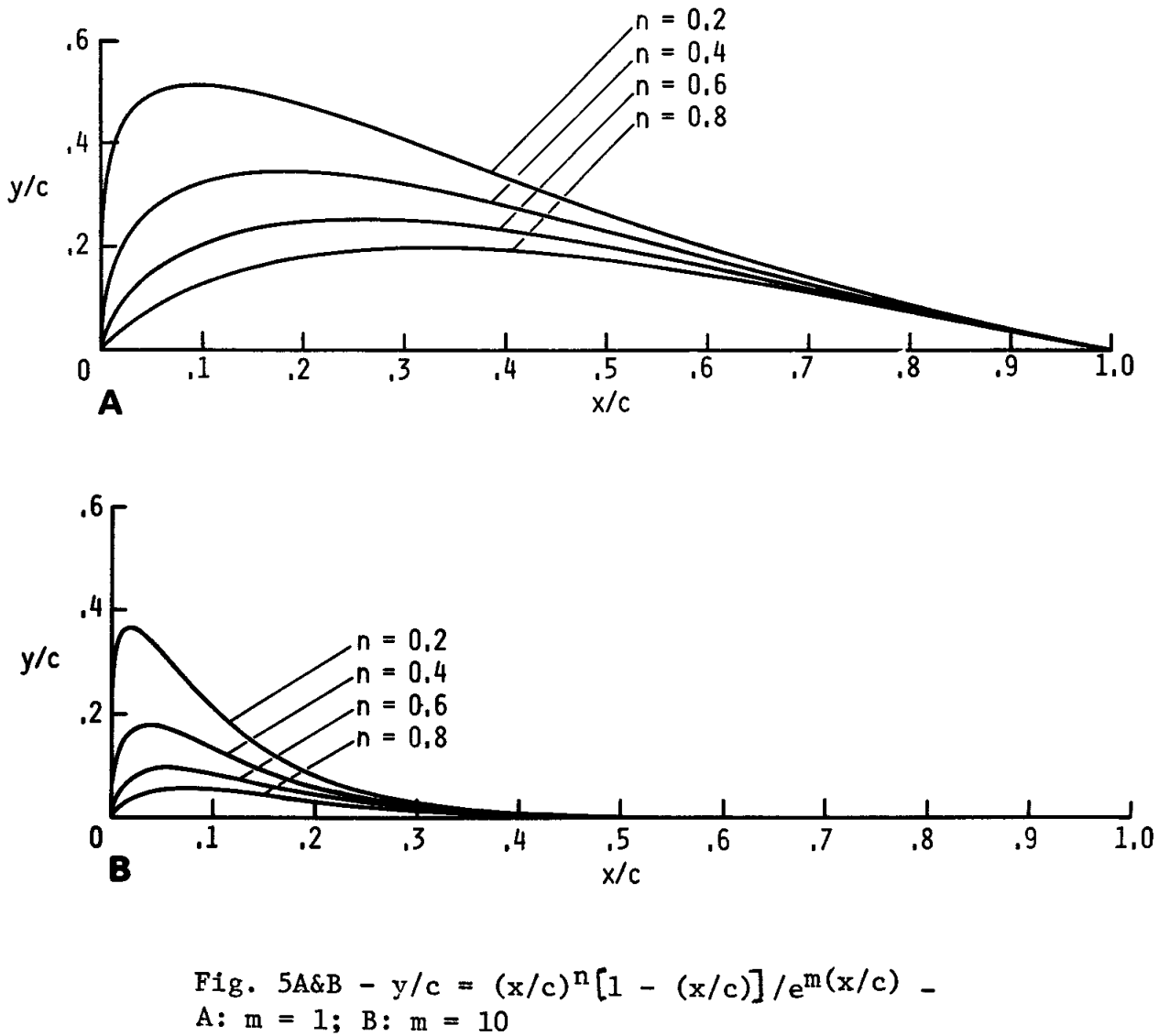
Graph showing polynomial-exponential basis functions for different $m$ and $n$ values. — Figure 1:Polynomial-exponential basis functions.

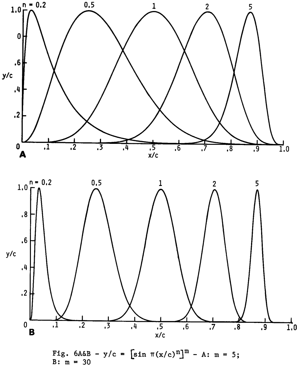
Graph showing sinusoidal basis functions for different $m$ and $n$ values. — Figure 2:Sinusoidal basis functions.

Implementation using `geodiff`¶

We now look at how geodiff allows us to easily use the Hicks-Henne parameterization to represent shapes.

The Hicks-Henne class initializer and its expected arguments are shown below:

hicks_henne.py

    def __init__(
        self,
        X_upper_baseline: np.ndarray | torch.Tensor,
        X_lower_baseline: np.ndarray | torch.Tensor,
        polyexp_m: float,
        polyexp_n_list: list[int],
        sin_m: float,
        sin_n_list: list[int] | None = None,
        sin_n_count: int | None = None,
    ) -> None:

To construct a Hicks-Henne object, we must supply:

Baseline coordinate for the upper and lower surfaces.
Parameters for the polynomial-exponential basis.
Parameters for the sinusoidal basis.

The implementation supports only a single exponent m for each of the basis class while allowing multiple n values to use different basis functions from a family.

Polynomial-exponential family: requires an explicit set of n values.
Sinusoidal family: can be specified in one of two ways:
- By providing an explicit list of n values, or
- By giving only the count of n values, in which case the code automatically constructs a list corresponding to count equally spaced sinusoidal peaks over the interval $[0,1]$ .

Fitting Shapes¶

We will use a circle as our baseline geometry and a square as our target. We then use the ChamferLoss to compute the geometric difference loss between the target shape and the shape represented by our Hicks-Henne parameterization. Since the implementation is written in PyTorch we can use the autograd capabilities to compute the gradients of the loss w.r.t. the Hicks-Henne participation coefficients and use an optimizer to modify our geometry.

We start by obtaining points on our shapes and normalizing them appropriately such that $x \in [0, 1]$ as assumed by the implementation.

# Get points on a circle (baseline curve) and square (curve to fit)
num_pts = 1000
X_circle = circle(num_pts)
X_square = square(num_pts)

# For Hicks-Henne x values should lie in the range [0, 1]
X_circle = normalize_0_to_1(X_circle)
X_square = normalize_0_to_1(X_square)

# Extract upper and lower coordinates for Hicks-Henne
idx_upper = X_circle[:, 1] >= 0
idx_lower = X_circle[:, 1] < 0
X_upper_baseline = X_circle[idx_upper]
X_lower_baseline = X_circle[idx_lower]

We now create a HicksHenne object by specifying the baseline coordinates and the parameters for the basis functions.

# Create a HicksHenne object
hicks_henne = HicksHenne(
    X_upper_baseline = X_upper_baseline,
    X_lower_baseline = X_lower_baseline,
    polyexp_m = 5,
    polyexp_n_list = [0.2, 0.4, 0.6, 0.8],
    sin_m = 5,
    sin_n_list = None,
    sin_n_count = 12
)

We use the ChamferLoss provided by geodiff to compute a geometric loss between the target shape and the shape represented by the HicksHenne object. PyTorch’s autograd capabilities then allow us to compute gradients of the loss w.r.t. the Hicks-Henne participation coefficients and modify them to fit the target shape.

# Train the Hicks-Henne parameters to fit the square
loss_fn = ChamferLoss()

learning_rate = 0.001
epochs = 1000
print_cost_every = 200

Y_train = X_square

optimizer = torch.optim.Adam(hicks_henne.parameters(), lr = learning_rate)
scheduler = torch.optim.lr_scheduler.ReduceLROnPlateau(optimizer, factor = 0.99)

for epoch in range(epochs):
    Y_model = hicks_henne()
    Y_model = torch.vstack([Y_model[0], Y_model[1]])
    
    loss = loss_fn(Y_model, Y_train)

    loss.backward()
    optimizer.step()
    optimizer.zero_grad()
    scheduler.step(loss.item())

    if epoch == 0 or (epoch + 1) % print_cost_every == 0:
        num_digits = len(str(epochs))
        print(f'Epoch: [{epoch + 1:{num_digits}}/{epochs}]. Loss: {loss.item():11.6f}')

Epoch: [   1/1000]. Loss:    0.011618
Epoch: [ 200/1000]. Loss:    0.000807
Epoch: [ 400/1000]. Loss:    0.000367
Epoch: [ 600/1000]. Loss:    0.000308
Epoch: [ 800/1000]. Loss:    0.000293
Epoch: [1000/1000]. Loss:    0.000289

We can now visualize the shape represented by our HicksHenne object using its visualize method.

# Visualize the fitted Hicks-Henne shape
fig, ax = hicks_henne.visualize()
plt.tight_layout()
plt.show()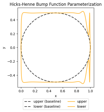

The polynomial-exponential functions are active close to $x = 0$ and therefore we get a better fit there compared to near $x = 1$ where only the sinusoidal family is active.

Footnotes¶

In mathematical analysis, a bump function (also called a test function) is a function $f: \mathbb{R}^{n} \rightarrow \mathbb{R}$ on a Euclidean space $\mathbb{R}^{n}$ which is both smooth (in the sense of having continuous derivates of all orders) and compactly supported.
Wikipedia, Bump function
In simpler terms, a bump function has derivatives of all orders and is only non-zero on a finite region, meaning it is “localized” and only modifies the shape within a specific interval.
↩
Figures adapted from Hicks & Vanderplaats, 1977.
↩

References¶

Hicks, R. M., & Henne, P. A. (1978). Wing design by numerical optimization. Journal of Aircraft, 15(7), 407–412.
Hicks, R. M., & Vanderplaats, G. N. (1977). Application of numerical optimization to the design of supercritical airfoils without drag-creep [Techreport]. SAE Technical Paper.

GeoDiff

CST - Class Shape Transformation

Hicks-Henne Bump Functions

Theoretical Background¶

Implementation using geodiff¶

Fitting Shapes¶

Implementation using `geodiff`¶