NIGnet - Neural Injective Geometry network

Neural Injective Geometry network (NIGnet) is a neural architecture proposed by Aalok & Alonso, 2025. It is a specially designed neural network architecture that is invertible and therefore provides a way of representing only non-self-intersecting geometry. We do this by using a Pre-Aux net with the NIGnet architecture. In this tutorial, we walk through the theory behind the NIGNet representation and how to actually use their geodiff implementation in practice.

# Basic Imports
import matplotlib.pyplot as plt
import torch

from geodiff.aux_nets import PreAuxNet
from geodiff.nig_net import NIGnet
from geodiff.monotonic_nets import SmoothMinMaxNet
from geodiff.loss_functions.chamfer import ChamferLoss

from assets.utils import square, normalize_0_to_1


# Set the seed for reproducibility
torch.manual_seed(42)

<torch._C.Generator at 0x116072150>

Theoretical Background¶

The NIGnet architecture as proposed in Aalok & Alonso, 2025 is based on the idea of stacking simple nonlinear invertible transformations. Computing the inverse and the determinant of the Jacobian is useful for log-likelihood training of generative models (of say images) but we do not require these properties and are only interested in the architecture being guaranteed invertible. That is, as long as we are concerned we only need a guarantee on the transformation represented by the network being invertible we will never actually want to invert it or compute the Jacobian of the determinant. Therefore, we only focus on the forward pass of the network and do not discuss the computations of the inverse or the determinant of the Jacobian.

The NIGnet architecture is composed of bijective transformations that serve as a building block for the entire transformation f. In particular, it uses linear layers followed by monotonic networks as the building block defined as follows:

Linear layer: To guarantee that the linear layers are invertible we use the matrix exponential.

\begin{align*} &W \in \mathbb{R}^{2 \times 2} \\ &A = e^{W} \\ &y = Ax \end{align*}

(1)

Since the matrix exponential returns an invertible matrix for any weight matrix $W$ , we can run unconstrained optimization on $W$ while guaranteeing non-self-intersection.

Monotonic layer: Let $x \in \mathbb{R}^{D}$ with its elements denoted by $x_i$ and $m$ be a monotonic function defined on $\mathbb{R}$ . The monotonic function is parameterized by a monotonic network and replaces the activation functions usually used in neural networks. Let $y$ denote the output of the monotonic layer with its elements denoted by $y_i$ . Then we have:

y_i = m(x_i) \qquad i = {1, \ldots, D}

(2)

Implementation using `geodiff`¶

We now look at how geodiff allows us to easily use the NIGnet parameterization to represent shapes.

The NIGnet class initializer and its expected arguments are shown below:

nig_net.py

    def __init__(
        self,
        geometry_dim: int,
        layer_count: int,
        preaux_net: nn.Module,
        monotonic_net: nn.Module,
        use_batchnormalization: bool = False,
        use_residual_connection: bool = True,
        intersection_mode: str = 'possible',
    ) -> None:

To construct a NIGnet object, we need to supply:

Geometry Dimension 2 for 2D and 3 for 3D.
Layer Count the number of layers in the NIGnet architecture.
Monotonic Net a torch network module to be used as the monotonic network.
Pre-Aux Net parameters such as layer count, hidden dimension, activation, normalization and output functions.
Boolean Flags for using batch normalization and residual connections with the NIGnet layers.
Intersection Mode to decide whether to use a Linear layer (possible intersection) or an ExpLinear layer (impossible intersection).

Fitting Shapes¶

We will use a square as our target geometry. We then use the ChamferLoss to compute the geometric difference loss between the target shape and the shape represented by our NIGnet parameterization. Since the implementation is written in PyTorch we can use the autograd capabilities to compute the gradients of the loss w.r.t. the NIGnet network parameters and use an optimizer to modify our geometry.

We start by obtaining points on our shapes and normalizing them appropriately such that $x \in [0, 1]$ . This is not needed for NIGnet but is used to offer a comparison with the classical shape representation methods like Hicks-Henne and CST.

# Get points on a square (curve to fit)
num_pts = 1000
X_square = square(num_pts)

# Normalize x values to the range [0, 1] to compare with other representation methods
X_square = normalize_0_to_1(X_square)

We now create a NIGnet object by specifying the geometry dimension, layer count, monotonic network and Pre-Aux net parameters.

# Create a NIGnet object
# First create Pre-Aux and monotonic networks to pass to the NIGnet initializer
preaux_net = PreAuxNet(geometry_dim = 2, layer_count = 2, hidden_dim = 20)
monotonic_net = SmoothMinMaxNet(input_dim = 1, n_groups = 6, nodes_per_group = 6)
nig_net = NIGnet(
    geometry_dim = 2,
    layer_count = 4,
    preaux_net = preaux_net,
    monotonic_net = monotonic_net,
)

We use the ChamferLoss provided by geodiff to compute a geometric loss between the target shape and the shape represented by the NIGnet object. PyTorch’s autograd capabilities then allow us to compute gradients of the loss w.r.t. the NIGnet network parameters and modify them to fit the target shape.

# Train the NIGnet parameters to fit the square
loss_fn = ChamferLoss()

learning_rate = 0.01
epochs = 1000
print_cost_every = 200

Y_train = X_square

optimizer = torch.optim.Adam(nig_net.parameters(), lr = learning_rate)
scheduler = torch.optim.lr_scheduler.ReduceLROnPlateau(optimizer, factor = 0.99)

for epoch in range(epochs):
    Y_model = nig_net(num_pts = num_pts)
    
    loss = loss_fn(Y_model, Y_train)

    loss.backward()
    optimizer.step()
    optimizer.zero_grad()
    scheduler.step(loss.item())

    if epoch == 0 or (epoch + 1) % print_cost_every == 0:
        num_digits = len(str(epochs))
        print(f'Epoch: [{epoch + 1:{num_digits}}/{epochs}]. Loss: {loss.item():11.6f}')

Epoch: [   1/1000]. Loss:    0.400921
Epoch: [ 200/1000]. Loss:    0.003428
Epoch: [ 400/1000]. Loss:    0.000974
Epoch: [ 600/1000]. Loss:    0.000243
Epoch: [ 800/1000]. Loss:    0.000100
Epoch: [1000/1000]. Loss:    0.000053

We can now visualize the shape represented by our NIGnet object using its visualize method.

# Visualize the fitted NIGnet shape
fig, ax = nig_net.visualize(num_pts = num_pts)
plt.tight_layout()
plt.show()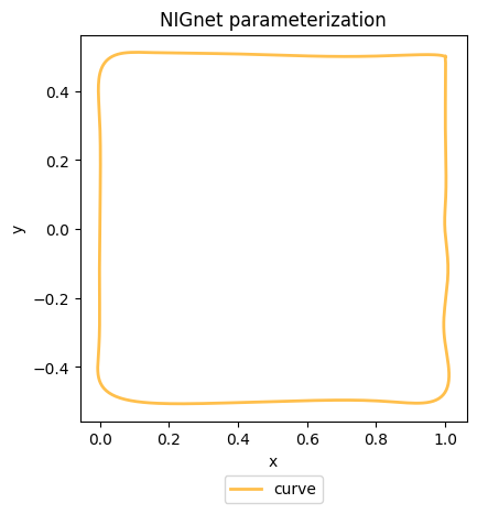

References¶

Aalok, A., & Alonso, J. J. (2025). NIGnets. https://github.com/atharvaaalok/NIGnets

GeoDiff

RealNVP - Real-valued Non-Volume Preserving

GeoDiff

NeuralODE - Neural Ordinary Differential Equations

NIGnet - Neural Injective Geometry network

Theoretical Background¶

Implementation using geodiff¶

Fitting Shapes¶

Implementation using `geodiff`¶